Multivariate

Overall workflow

This tool supports threshold setting for nutrients and other supporting physico-chemical elements when ecological status is influenced by more than one stressor. The workflow follows the multiple-stressor guidance: choose a suitable Biological Quality Element, screen candidate stressors, build transparent logistic models, evaluate classification thresholds, and then predict boundary values under realistic combinations of other pressures.

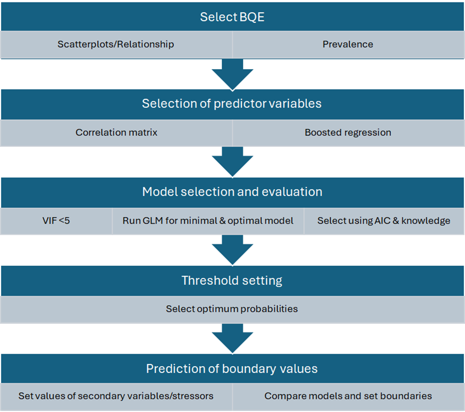
How the left-hand menu follows the workflow

Step 1: Data import - load the example dataset or upload a wide-format CSV file, then check variable names and data structure.
Step 2: Analysis setup - select the EQR/BQE response, set the Moderate-Good EQR boundary, choose the shared predictor set, and inspect density, Q-Q, and normality diagnostics.
Step 3: Univariate screening - inspect the relationship between one stressor and the response, including the binary good-or-better classification and univariate diagnostics.
Step 4: Predictor screening BRT - use boosted regression trees to rank predictors and inspect partial dependence patterns.
Step 5: Predictor screening SEM - fit path models, review direct effects, and inspect covariance/correlation structure among selected variables.
Step 6: Multivariate models - fit GLM models using the shared predictor set, compare model support, check VIF/Cook's distance, and inspect effects and PCA plots.
Step 7: Thresholds & boundaries - solve candidate boundary values from the selected multivariate model and export the report.

Statistical workflow

Select BQE and data: use an ecological response with enough observations and a balanced number of sites above and below the boundary of interest.
Univariate screening: check the direct relationship between the BQE/EQR and each stressor, including the binary good-or-better classification used by the logistic models.
Predictor screening: use BRT importance, BRT partial dependence, SEM paths, normality checks, and correlation warnings to identify informative and ecologically plausible predictors.
Multivariate modelling: compare minimal, full, optimal, and additional candidate GLM models. Prefer models that improve explanatory power without unnecessary complexity.
Thresholds and boundaries: choose a probability cut-off using kappa, omission, and commission errors, then solve for boundary values while holding other stressors at selected values.

How to interpret the outputs

The app does not replace ecological judgement. It generates candidate boundaries and diagnostic evidence. Final values should be selected with knowledge of local pressures, typology, feasibility of management actions, and stakeholder or expert consultation.

Highly correlated predictors can destabilise model coefficients; the guide recommends avoiding pairs with |r| greater than 0.7 in the same final model.
Typological variables, non-manageable stressors, and manageable stressors should be treated differently when fixing values for boundary prediction.
Boundary predictions should usually stay within the interquartile range of supporting predictors, because extrapolation near distribution extremes is less reliable.
For multivariate models, balanced omission and commission errors are often more appropriate than a strongly precautionary univariate cut-off.
The final boundary should be checked against other evidence, other BQEs where available, and national or regional ecological knowledge.

References and guidance

The workflow implemented in this app follows the ECOSTAT/JRC guidance for setting nutrient and supporting-element boundaries under multiple-stressor conditions. The references below provide the methodological background for BQE selection, predictor screening, logistic modelling, threshold selection, and final ecological interpretation.

Phillips, G., Kelly, M.G., Teixeira, H., Free, G., Varbiro, G., Varkitzi, I., Lazaridou, M., Ntislidou, C., Karaouzas, I., Kolada, A., Folster, J. and Mingarelli, S. Checking and setting nutrient criteria to support ecological status. iii. Setting nutrient criteria when other stressors are present. ECOSTAT / JRC guidance document draft, 2026.
Phillips, G., Kelly, M., Teixeira, H., Free, G., Varbiro, G., Varkitzi, I., Kolada, A., Lyche Solheim, A., Poikane, S. Best practice for establishing nutrient concentrations to support good ecological status, revised guidance, 2026.
Phillips, G., Kelly, M., Teixeira, H., Salas, F., Free, G., Leujak, W., Pitt, J.-A., Lyche Solheim, A., Varbiro, G. and Poikane, S. Best practice for establishing nutrient concentrations to support good ecological status. Publications Office of the European Union, 2018/2019.
Kelly, M.G. and colleagues. Toolkit and mismatch-method guidance for deriving nutrient boundaries from ecological classification models, including omission, commission, kappa and probability-threshold diagnostics.
Feld, C.K. and colleagues. Guidance and routines for analysing multiple stressors, biological responses and ecological assessment data.
Elith, J., Leathwick, J.R. and Hastie, T. A working guide to boosted regression trees. Journal of Animal Ecology, 2008.
Burnham, K.P. and Anderson, D.R. Model Selection and Multimodel Inference: A Practical Information-Theoretic Approach. Springer, 2002.
Fox, J. and Monette, G. Generalized collinearity diagnostics. Journal of the American Statistical Association, 1992.
Rosseel, Y. lavaan: An R package for structural equation modeling. Journal of Statistical Software, 2012.

References are included to document the scientific basis of the workflow. Final boundary values should still be selected with local ecological knowledge and expert consultation.

Import

Select the proper separator and decimal settings before loading the data.

Data should be in wide format: one sampling record per row, with the ecological response or EQR column and each stressor or predictor in separate columns.

Example file structure

site_id	waterbody_type	EQR	Total_P	Total_N	Conductivity
Lake_001	lowland	0.72	28.4	1.10	365
Lake_002	upland	0.48	63.1	1.85	510

Use numeric columns for the EQR/response and stressors. Existing binary status columns can also be used in Step 7.

Separator

Comma

Semicolon

Tab

Decimal

Comma

Point

Tools

Choose CSV File

Browse...

*In order to test the application .... Download empty data template

Content of the datafile

Description of the data file

Data structure check

Variables

Summary

Shared analysis setup

Select the ecological response and the common predictor set once here. The univariate, BRT, SEM, multivariate, and boundary tabs all use these shared settings so the workflow stays consistent.

EQR / BQE response column:

Shared stressor / predictor variables:

These selected variables are used by BRT, SEM defaults, correlation, normality checks, VIF, PCA, multivariate GLM, and threshold diagnostics.

Apply log10 to shared predictors:

Use log10 for positive, right-skewed stressors such as nutrients or conductivity. The app creates transformed model variables internally and keeps the original column names unchanged.

Normality and transformation screening

Use these diagnostics in the setup step to decide which shared predictors should be log10-transformed before BRT, SEM, multivariate GLM, and boundary modelling.

Density plots: These show the empirical distribution of each predictor. A roughly symmetric, bell-shaped curve suggests approximate normality. Strong right-skew is common for nutrients.

Q-Q plots: Points should fall along the 45 degree reference line if the data follow a normal distribution. Curvature indicates skewness; S-shaped patterns suggest heavy tails.

Shapiro-Wilk test: Tests the null hypothesis that the data are normally distributed.

p >= 0.05: no strong evidence against normality
p < 0.05: significant deviation from normality

With larger sample sizes, the Shapiro test becomes very sensitive. Always interpret the test together with the density and Q-Q plots.

Practical guidance for modelling: Logistic regression and classification models do not require normally distributed predictors, but severe skewness may affect interpretability or model stability.

Consider log10 transformation for right-skewed environmental variables.
Check whether transformation improves symmetry and Q-Q alignment.
Avoid over-transforming variables with already symmetric distributions.

Univariate Settings

The univariate step fits one stressor at a time against the selected ecological response. Use this to screen individual pressure-response relationships before building a multivariate model. The EQR column is converted to a binary class using the selected boundary. Sites at or above the boundary are treated as good or better; sites below it are treated as below good status.

Predictor variable:

Apply log10 transform

Use log10 transformation for strongly right-skewed stressors such as nutrients or conductivity. The transformation is applied only to the selected predictor in this univariate model.

Univariate Logistic

The logistic plot shows how the probability of good-or-better ecological status changes along the selected stressor gradient. A steep curve indicates a narrow stressor range where classification probability changes rapidly.

This plot shows the relationship between the selected stressor and the probability that a site is classified as good ecological status or better. Each point represents an observed site, while the line shows the fitted model response. The curve illustrates how the likelihood of achieving good ecological condition changes along the stressor gradient. A steep decline in the curve indicates a range where increasing stressor levels are associated with a rapid decrease in the probability of good ecological status.

The lower plot compares the original EQR values with the selected stressor. The dashed line marks the EQR boundary used to create the binary class; the smooth line is a descriptive trend, not the classification model itself.

Relationship between Biological metric(EQR) and stressor concentration, dotted lines mark biota good/moderate boundary. Blue lines show GAM model fit to illustrate the general trend.

Thresholds

This table evaluates probability thresholds for converting fitted probabilities into binary predictions. Sensitivity measures how many good-or-better sites are correctly detected; specificity measures how many below-good sites are correctly detected.

ROC / AUC

The ROC curve summarizes discrimination across all probability thresholds. AUC close to 1 indicates strong separation between classes; AUC near 0.5 indicates little discrimination.

Shared predictors used here

The multivariate step fits the shared predictor set selected in Step 1. This helps identify stressors that remain informative after accounting for the other selected variables. To change the response column, predictor list, or log10 transformations, return to Step 2: Analysis setup. Additional variables in the uploaded file are ignored unless selected in the shared setup.

Correlation (EQR + selected predictors)

The correlation heatmap and table show pairwise association among the response and selected predictors. Strong correlations between predictors can indicate redundancy or multicollinearity. Pearson is sensitive to linear relationships and outliers. Spearman and Kendall are rank-based and often more robust for monotonic ecological gradients.

Method:

Use log10 for selected predictors (if set in MV)

VIF (multicollinearity) for selected predictors

VIF quantifies how strongly each predictor can be explained by the other predictors. High VIF values indicate multicollinearity, which can make coefficients unstable even when model predictions look reasonable. Cook's distance highlights observations with high influence on the fitted model. Investigate influential sites before interpreting coefficients or thresholds.

Coefficients

Model coefficients from the fitted multivariate model.
Estimates are shown with standard errors, test statistics and p-values (rounded to 3 decimals). Positive coefficients increase the probability of good-or-better status; negative coefficients decrease it, conditional on the other selected predictors.

Model selection

The model selection table compares subsets of the selected predictors using information criteria. Lower AIC values indicate better expected predictive support after accounting for model complexity. The candidate model panel follows the guide terminology: minimal uses the first selected predictor as the primary stressor, full uses all selected predictors, optimal is the lowest-AICc subset from MuMIn, and additional is the full model when it differs from the optimal model.

Effects

The effects plot shows fitted probability patterns for one selected predictor while using the multivariate model. Use it as a visual summary of model behaviour, not as a substitute for coefficient and threshold checks.

PCA

The PCA plot summarizes multivariate structure in the selected predictors. It can reveal gradients, clusters, and outlying sites, but it is exploratory and separate from the logistic model.

Multivariate boundary prediction

What this step does: estimates the value of a primary stressor that corresponds to a selected probability of good-or-better ecological status, while accounting for other pressures.

Example: to estimate TP boundaries at different levels of AbsF, select EQR as the response, TP as the primary stressor, and AbsF as the secondary stressor. Leave the additional stressor fields set to None.

1. What boundary do you focus?

Biological response

Select a numeric EQR/BQE metric or an existing binary good/below-good class.

Biological response boundary (Moderate / Good)

Used only when the selected response is numeric. Values at or above this boundary are classified as good or better.

Primary stressor: calculate boundary for

This is the pressure in focus for which the app will calculate a candidate boundary, for example TP.

2. How should other pressures vary?

Secondary stressor: compare levels of

Required. The app calculates the primary-stressor boundary at representative levels of this pressure; these levels form the table rows.

Additional stressor: compare across columns (optional)

Optional. Select this only when boundaries should also be compared across a second pressure.

Additional stressor: hold at representative values (optional)

Optional. Use this for a further predictor to be held at representative values; otherwise leave it as None.

3. Model options

Probability of good-or-better status

The app solves for the primary-stressor value at this fitted probability. This is not the nutrient boundary itself.

Variables modelled on log10 scale

Also fit univariate comparison model

Advanced output setting

Output column prefix

Optional. Leave blank to use an automatic prefix based on the primary stressor.

Download XLSX report

Model summary

The model summary lists selected variables, model formula, transformed variables, fitted coefficients, AIC values, and AUC/prevalence where available. Use this section to confirm the app fitted the intended model.

Boundary prediction tables

Boundary tables show the calculated primary-stressor boundary across representative levels of the selected secondary and optional additional stressors. Values are rounded for display; exported long-format results retain full precision. The required secondary stressor forms the table rows. If selected, the additional comparison stressor forms columns, while the conditioning stressor is held at representative values.

Threshold curves (kappa, omission & commission)

These curves show how classification metrics change as the probability threshold changes. Kappa summarizes agreement beyond chance; omission is false negatives; commission is false positives. The optimal threshold table reports several candidate threshold rules. Different rules emphasize different trade-offs, so the ecological and management context should guide the final choice.

Boundary probability curve

The probability curve shows the fitted response along the boundary stressor while other selected stressors are held fixed. Vertical reference lines mark solved univariate and multivariate boundaries when available.

Structural equation model

SEM fits a path model among the selected numeric variables. Use the response as the ecological endpoint and predictors as stressors or supporting environmental variables. SEM uses the shared response and predictor variables selected in Step 1. With automatic syntax enabled, the model estimates direct paths from all selected predictors to the response and allows predictors to covary with each other. You can turn this off and edit the lavaan syntax manually for more specific causal hypotheses.

Standardize selected variables before fitting

Use automatic multivariate path model

SEM path diagram

The SEM path diagram shows the fitted relationships as arrows. Arrow labels are standardized coefficients when standardization is enabled: larger absolute values indicate stronger direct associations, positive values indicate increasing relationships, and negative values indicate decreasing relationships. Curved double-headed links represent covariance between predictors. The diagram is descriptive and model-based; ecological interpretation still depends on whether the specified paths are biologically plausible.

Direct effects on the response

This plot extracts the direct SEM paths pointing to the ecological response. Bars show standardized coefficients: green values indicate positive associations with the response, red values indicate negative associations, and longer bars indicate stronger direct effects. Use this view when the network diagram is crowded and you mainly need to compare which stressors have the strongest direct modelled relationship with the response.

SEM variable correlation heatmap

This heatmap shows Pearson correlations among the variables used by the SEM after the same filtering and standardization choices. Darker colours indicate stronger positive or negative relationships. Use this view to understand the covariance links in the path diagram and to spot predictor pairs that may carry overlapping information.

Model summary

The model summary reports lavaan estimates, standard errors, significance tests, standardized coefficients, R-squared values, and global fit statistics.

Standardized paths and fit measures

The paths table lists estimated regression paths and covariances. Key columns are est, pvalue, and std.all. The fit table gives common SEM diagnostics such as CFI, TLI, RMSEA, SRMR, AIC, and BIC.

BRT Importance

Boosted Regression Trees are used here to estimate the relative influence of selected predictors on the ecological response. BRT can capture nonlinear relationships and interactions that may be missed by simpler regression models. BRT uses the shared response and predictor variables selected in Step 1. The importance plot ranks predictors by their contribution to reducing prediction error across the fitted tree ensemble. Higher values indicate variables that were used more often and more effectively in the boosted trees.

Model Output

The BRT model output reports fitting settings, model performance, selected tree complexity, learning rate, number of trees, and relative influence values. Use these diagnostics to judge whether the model is stable enough to interpret. BRT importance is not a causal estimate. Interpret high-ranking variables as strong predictive signals, then compare them with the multivariate model, threshold results, and ecological knowledge.

BRT partial dependence

Partial dependence plots show the fitted BRT response for one predictor while averaging over the other predictors. They are useful for spotting narrow response ranges, nonlinear effects, and variables that may benefit from log10 transformation before GLM modelling. The y-axis is the model partial effect on the BRT scale, so use the shape and turning points rather than the absolute value. These plots support predictor screening; they do not replace the GLM boundary model.

Overall workflow

How the left-hand menu follows the workflow

Statistical workflow

How to interpret the outputs

References and guidance

Geoff Phillips

Freshwater ecologist

Martyn Kelly

Diatom & river assessment expert

Heliana Teixeira

Marine & freshwater indicators

Gary Free

Lake ecology & WFD expert

Agnieszka K. Kolada

Macrophyte assessment expert

Sandra Mingarelli

EU WFD coordination expert

Várbíró Gábor

R & Shiny developer

Import

Content of the datafile

Description of the data file

Data structure check

Variables

Summary

Shared analysis setup

Normality and transformation screening

Univariate Settings

Univariate Logistic

Thresholds

ROC / AUC

Shared predictors used here

Correlation (EQR + selected predictors)

VIF (multicollinearity) for selected predictors

Coefficients

Model selection

Effects

PCA

Multivariate boundary prediction

1. What boundary do you focus?

2. How should other pressures vary?

3. Model options

Model summary

Boundary prediction tables

Threshold curves (kappa, omission & commission)

Boundary probability curve

Structural equation model

SEM path diagram

Direct effects on the response

SEM variable correlation heatmap

Model summary

Standardized paths and fit measures

BRT Importance

Model Output

BRT partial dependence